Topic modelling clickbait headlines with Python
Very often I come across business problems where a large amount of natural language data needs to be processed and analysed. For example:
Document review for legal investigations - Tens of thousands of emails must be reviewed for a legal investigation. Which subset of those emails should be looked at first?
Penetration test reports - Using several years of regular penetration test reports for hundreds of individual applications, what are the most prevalent issues across the organisation?
Spend categorisation - A company has individual line item descriptions for millions of transactions made for their business. How can they work out sensible categories for what they are spending money on?
One good starting point for the problems is to build a topic model. The aim of a topic model is to find abstract topics within a collection of documents. Topic modelling can reveal hidden structure in large bodies of text. Structure allows us to better understand the information within the data and make better business decisions as a result.
Topic modelling can often be approached the same way for different business problems, so having a write-up post with accompanying code is hopefully a useful resource. We will go over the following:
How to prepare the text data for topic modelling;
Extracting the topics from the data with non-negative matrix factorisation (NMF);
Working out a summary for each topic;
Determining the optimal number of topics; and
Predicting the topic of a new document.
All of the code for this post can be found on my GitHub.
Business problem
We are a newly hired data scientist at a tabloid newspaper that has recently moved to an online publication model. As a new player in the online media space, they want to get a better understanding of what their competitors write about. The editor has some idea of the types of content that are popular (quizzes, celebrity gossip, animals) but wants a more detailed, data-driven breakdown of the topics that feature most prominently on other sites.
Data
To demonstrate topic modelling, we are using a dataset released for the paper Stop Clickbait: Detecting and Preventing Clickbaits in Online News Media. The data consists of consists of 16,000 article headlines from ‘BuzzFeed’, ‘Upworthy’, ‘ViralNova’, ‘Thatscoop’, ‘Scoopwhoop’ and ‘ViralStories’.
The dataset is relatively small (less than 1MB) so we will load it into our Google Colab notebook with Google Sheets.

We’ve seen a few examples of the clickbait headlines. Let’s have a look at some summary statistics to get more familiar with the data.
Clickbait headline word count distribution
The average title word count is 9, with a fairly normal looking distribution.
Text Processing
Before we can run our topic clustering algorithm, we need to process and clean the text data. The techniques to process text will be different for each business problem. We’ll go over some of the most common methods below:
Tokenisation involves breaking up a sequence of strings into pieces, called tokens. Generally punctuation is discarded from each token.
Lower-casing the text ensures words with different capitalisation are treated the same way by the algorithm.
Expanding contractions changes words like can’t to can not consistently for all of the clickbait titles.
Removing stopwords like the, is and of ensures that we only keep words with useful information for our topic model. We also remove all punctuation, spaces and words shorter than 2 characters.
The full code for the text processing can be found here, adapted from R Salgado’s code.
The aim of text processing is to increase the algorithm’s ability to detect topics within our data. Let’s look at the top 20 words by frequency, after we have processed our text:
Top 20 words by frequency
It looks like there may be a few common themes in the headlines. The words ‘people’, ‘things’ and ‘times’ occur often, suggesting many of the headlines are lists of those subjects. Word frequency often doesn’t tell us a lot about the dataset, but it does confirm that our text processing step was mostly successful.
Word vectorisation with tf-idf
The last data processing step before we generate our topic model is to convert the text to a more manageable representation for the algorithm. Natural language processing algorithms cannot process the headlines in their original form. Instead, the algorithms expect numerical feature vectors with a fixed size. Text vectorisation is the process of converting text into a numerical representation.
Examples of techniques for text vectorisation include bag-of-words and word2vec. For each term in our dataset, we will calculate a measure called Term Frequency, Inverse Document Frequency, abbreviated to tf-idf. The technique provides a statistic that is intended to reflect how important a word is to a document within the corpus. From Wikipedia:
The tf–idf value increases proportionally to the number of times a word appears in the document and is offset by the number of documents in the corpus that contain the word, which helps to adjust for the fact that some words appear more frequently in general.
We will use the class sklearn.feature_extraction.text.TfidfVectorizer to calculate a tf-idf vector for each of the headlines.
Words that occur very commonly or very infrequently in our corpus will not improve the quality of our topic model, so we exclude them. The min_df argument tells the function to ignore any words that occur in less than 5 of the headlines. max_df tells the function to exclude words that show up in more than 80% of the headlines.
After the text processing step, our corpus had just under 12,000 unique words. The topics are likely to be made up of the more frequently occuring words, so will will set the max_features to 6,000.
The vectoriser also gives the option to create vectors for n-grams. Setting ngram_range to (1, 2) will create unigram and bigram weights. Bigrams may be useful for words that often are found together, for example ‘Harry’ and ‘Potter’.
Finally, preprocessor strips the individual n-grams from the lists in the dataframe column.
Extracting the topics from the data with non-negative matrix factorisation (NMF)
NMF takes a vectorised representation of the documents and words in our corpus and decomposes the representation into from high-dimensional vectors into a lower-dimensional representation.
We have 16,000 documents (headlines), and 6,000 unique vectorised n-grams. NMF decomposes the high-dimensional representation of the documents into a lower-dimensional representation made up of two matrices, W and H.
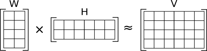
If we set the number of topics to 8, we would get the following matrices:
Original matrix
V = 16,000 x 6,000
Topic matrix
W = 8 x 6,000
Headlines by topic matrix
H = 16,000 x 8
The NMF model changes the values of the W and H matrices so that their product approaches V.
The topic number 8 was selected arbitrarily. Later on we can set the ‘optimum’ number of topics using the coherence score. With the headlines processed and the text vectorised, we can now run NMF.

NMF gives us the top words associated with each topic. Inspecting the 8 topics above, we can see some clear themes like ‘Harry Potter’ and social media sites. Some are less precise, like topic 4. Let’s see if we can improve the topic model by finding the best number of topics and comparing topic quality.
Selecting the optimal number of topics with the coherence score
The coherence score provides a measure for the degree of semantic similarity between high scoring words in a topic. A high scoring topic is one that is semantically interpretable. A set of words in a topic is coherent if the words support each other to give a clear context - i.e. telling us what kinds of headlines the topic covers. Topic coherence is a big subject, and is explained in better detail in the gensim package documentation.
Unfortunately, sklearn doesn’t give us the ability to generate coherence scores, so we need to run NMF with gensim. We could have used gensim from the beginning, but gensim only allows for a simple bag-of-words text representation, rather than the tf-idf vectorisation which we prefer. We can use the optimum number of topics from the gensim coherence score to rerun the NMF with our original approach.
The full code for generating the coherence score can be found on my GitHub. We can see the results for different numbers of topics below:
Coherence score by number of topics
For this particular dataset, the coherence score appears to increase with the more topics we include. It’s unclear whether this is a result of the dataset itself, or perhaps the representation of the data within the gensim NMF model. We don’t see a dramatic increase after 40 topics, so we’ll try the new topic value and look at the results.
Understanding the output of the topic model
Supervised learning algorithms give clearly interpretable outputs, as the inputs used to train them are already known e.g. ‘dog’, ‘cat’ or ‘fraud’ ‘not fraud’. The difficulty with unsupervised methods like NMF is that we essentially need to ‘eye-ball’ the results and use the words associated with each topic to come up with a label for that topic. Some are pretty clear, like ‘Disney’ and articles related to food:

Others are harder to interpret - topic 4 appears to be about social media related topics and also ‘lists of things’ or ‘times something happened’. Let’s link the topics back to the original documents and see how frequently each topic occurs, according to the NMF model:

The large number of vague topics is not surprising, as topic modelling on real data often produces similar results. Topic modelling is rarely a silver bullet for instantly understanding the composition of a set of documents. The initial expectation is that they will give a series of clear, accurate and easy to interpret topics. Often however, the data is noisy and sometimes lacking a clear division between documents and their associated topics. Unsupervised techniques like NMF can give us a good starting point for more targeted analysis and modelling. For example, the topics can be assessed and cherry picked for manual human classification. With an accurately labelled dataset, we can train supervised models to classify new documents into our chosen topics.
Final thoughts
Our initial business problem was to assess the Daily Cornet’s competitor headlines to see what kind of subjects were popular. Looking at the frequency of topics within the dataset confirmed some initial assumptions that quizzes, celebrity gossip and animals were popular topics. Articles related to social media sites, food and cooking were also common. To present the results to management, we would pick out coherent topics with a high frequency. We can then present a visual representation of the frequency of each of the topics. For example:
Distribution of topics in headlines
Hover over the segments to see the topics
Topic modelling can help to explore a text dataset for the first time. It can also give a good starting point for determining labels for a machine learning classifier. While the results are not always easy to interpret, NMF is a useful technique for exploring natural language problems.