Building a quantitative cyber-risk model in Python
In the previous post, we looked at some of the limitations of some of the widely used techniques for measuring cyber security risk. We explored how replacing risk matrices with more quantitative approaches could unlock a whole new class of decision making.
The steps below show how we can generate a loss exceedance curve with Monte Carlo simulations in Python. To show how the process works, we'll consider a scenario where a large online retailer wants to know if it's worthwhile to invest in cyber awareness training, or start a project to implement better security controls on their systems.
Our quantitative approach to measuring risk makes the following assumptions:
Risk from cyber security breaches can and should be measured in the same way that insurance companies and pension fund managers measure their risk. Rather than stating a risk is 'low', 'medium' or 'high', we should state time-framed probabilities. For example, there is a 10% chance of the company experiencing a customer data breach in the next year.
Estimates for loss should be made in dollar amounts. But instead of simple point-estimates (e.g. 'severe') the loss should be stated as a range of values within a credible interval. The credible interval allows room for uncertainty, and the many possible loss events that could happen.
Even with a small amount of data, experts can make quantitative estimates to help achieve what we're trying to do - ultimately make better, more educated decisions about cyber security risk management.
Cyber threat: Ransomware Attack
To understand the total risk exposure of a company, we need to work out what plausible cyber threats (events where a company asset is harmed) apply to the company's assets. This gives us a portfolio of 'cyber risks'. Cyber threats and cyber risks are subtly different. A threat is a potential event where a key asset could be harmed. For example, a ransomware attack on systems running an online retailer's e-commerce site. The cyber risk would be the likelihood of the event occurring, and the monetary loss that would result.
Probability: How likely is it that we get hit with a ransomware attack?
Consider two approaches to expressing the probability of a ransomware attack:
Qualitative approach: The likelihood of a ransomware attack is medium.
Quantitative approach: Based on the reported statistics of similar companies in our industry, and our existing controls, we estimate that the probability of experiencing a ransomware attack in the next year is 20%.
The quantitative approach gives us a number that we can use in a simulation. Before we simulate the attack, we need to express what we think the impact, or loss resulting from the event will be.
Impact: How much is it going to cost if our systems are infected with ransomware?
Qualitative approach: The impact of a ransomware attack would be high.
Quantitative approach: If a ransomware attack happens, there is a 90% chance that we will experience a loss between $50,000 and $250,000. We base this estimate on the potential lost sales if we were able to restore the systems from backups within 24 hours. The upper end of the estimate is based on ransoms paid, lost sales from system outages and reputational damage.
Isn't it impossible to measure reputational damage?
Reputational damage is often seen as unmeasurable, but there are good proxies for measuring potential financial loss from reputation damage. Think about what a company spends to improve their reputation - advertising. Reporting a major cyber breach would damage reputation, significantly decreasing the effect of previous money spent on advertising. Loss of sales compared to a previous period is another easily comparable metric.
Simulating a year of operation
First, we'll write some Python code to simulate a single year of operation. The simulation of ransomware attack risk is based on our estimates above. The first step is to generate a random number between 0 and 1. If the number is below 0.2 (our 20% probability) we can say that the ransomware attack happened.
Next we need to work out how much money was lost. This part is slightly more complex, as the losses between $50,000 and $250,000 are not all equally likely. It's more likely that losses are skewed towards the lower end. Huge losses, while possible, happen less frequently. A probability distribution expresses the range of values given by our expert, and the likelihood of each loss amount. The log-normal distribution is ideal for representing the probabilities associated with each possible loss amount.
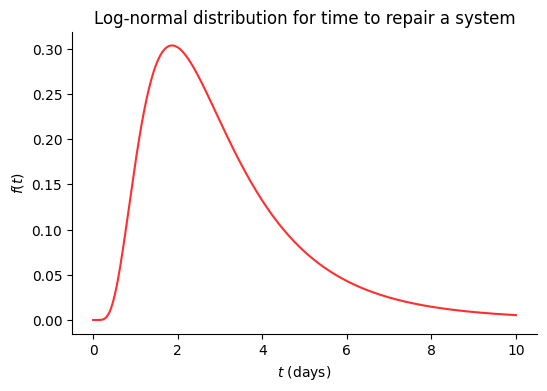
Here we have an example of a log-normal distribution that shows the different probabilities of 'time to repair a system'. We can see that the most likely value is around 2 days, while 8-10 days falls on the less likely end of the distribution.
But how can we make the distribution fit our 90% credible interval for loss? The probability density function for the log-normal distribution is:

where
σ is the standard deviation of normally distributed log of the variable.
μ is the mean of the normally distributed log of the variable.
The formula to derive μ and σ from the upper and lower estimates is given by:
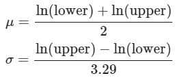
μ is calculated by taking the natural logs of the upper and lower estimates, and dividing by 2. We would do the same for a normal distribution, but wouldn't take the natural logs of the estimates.
For σ we divide by 3.29, as 90% of the values fall within 3.29 standard deviations of the mean of a normal distribution. We take the natural log of the upper and lower bounds to get σ for the log-normal distribution.
Let's plot the estimates from our ransomware example to see if the resulting distribution makes sense:

The distribution plot looks similar to our credible interval specification, with 90% of the area under the graph between $50,000 and $250,000. You may have noticed that the values for f(x) are smaller compared to the first example. The reason is that the total area under the curve for any probability distribution must add up to 1. As the values along the x-axis are relatively larger, f(x) must be equivalently smaller so that the total area adds to 1.
Using the Python NumPy library, we can get a simulated loss amount from the log-normal distribution:
We now have two functions that allow us to simulate the risk of a ransomware attack. Now we can see what a year of operation simulated 20 times looks like:
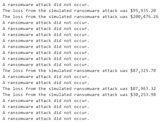
Twenty data points isn't really much to work with. It certainly wouldn't be enough data for something like training a machine learning algorithm. Fortunately we have the computing power to simulate the risk several thousand times, and see the distribution of losses. This is the core idea of Monte Carlo simulations, which we'll demonstrate in the chart below.
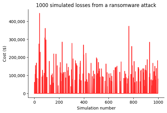
The average loss across the 1000 simulations was around $23,000. The gaps between the larger spikes represent simulations where a ransomware attack didn’t occur, resulting in a $0 loss value. We want to be able to quantify how certain we are about the $23,000 figure. Some simulations showed a loss of over $400,000. How certain are we that $23,000 is the most likely loss amount?
To express the probabilities of different losses, we can build a loss-exceedance curve. In simple terms, the loss-exceedance curve expresses the proportion of the total simulations run that are below a particular loss amount.

We can now ask questions of the graph such as:
What is the probability that we lose more than $50,000 from ransomware attacks in a year?

Reading from the graph again, we can see that there is an 80% chance of losing more than $23,000 from a ransomware attack in a year.
Building a cyber risk portfolio
So far, we've only considered a single cyber risk. Our hypothetical online retailer is exposed to many cyber risks. The method above can easily be expanded to a portfolio of possible cyber loss events. With each risk quantified, they can be combined into a single loss-exceedance curve to understand the total cyber risk exposure. Let’s add in a few more possible cyber events, along with the probability and loss estimates for a single year.

Similar to the example above, we will simulate each individual event and combine the total loss amounts for each year of simulation.
Plotting the individual losses for each of the 10,000 simulations gives:

The average loss in a simulated year was $94,120 for the portfolio of cyber risks. Plotting the loss-exceedance curve again:
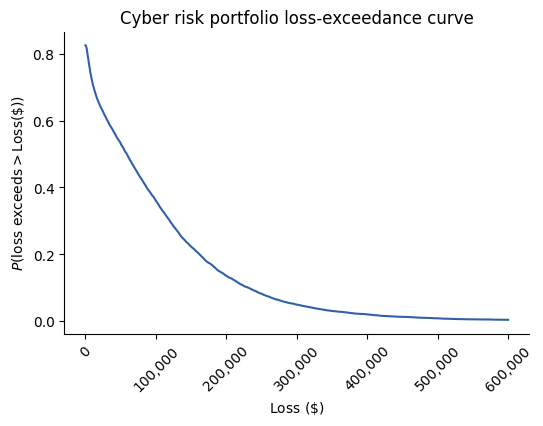
In the last post, we looked at how a 'risk tolerance' curve can be drawn from a few simple questions with management. Let’s add a risk tolerance curve to our loss-exceedance curve plot to compare the two.

To better understand the ‘problem area’, we can compare the values on the two curves. Management has stated that they will accept a 20% chance of losing more than $130,000 from all cyber risk events in any given year. The inherent risk analysis has shown that there is a 20% chance of losing more than $175,000 in a year. This is beyond the risk appetite of the company. They will likely want to compare potential mitigation actions to bring the inherent risk down.
How much should be spent on cyber-risk mitigation?
Let’s review the cyber risks and see what possible mitigation actions are available:
Ransomware employee awareness training
Cost: $25,000
Estimated risk mitigation: Probability of ransomware attack reduced from 20% to 10%.
Project to increase password complexity requirements
Cost: $30,000
Estimated risk mitigation: Probability of password cracking reduced from 40% to 10%.
Our first priority is to bring the inherent risk curve in line with the risk tolerance. We also want to consider the return on investment of each mitigation action. We can do this by re-running the simulation with each mitigation in place and seeing how the risk curves compare with the risk tolerance..
Comparing the area under the curve pre and post mitigation will give the difference in expected losses. The difference can be used to calculate the return on control.

We can add the points along the loss-exceedance curves to the function below to work out the area under the curve. The area is equivalent to the expected losses in any given year.
Expected loss in a year (inherent risk) = $94,120
Expected loss in a year (employee training mitigation) = $80,717
Expected loss in a year (increasing password complexity) = $58,118
Employee training ($25,000 cost)
Return on control = (($94,120 - $80,717) / $25,000) - 1 = -46.4% return
Increase password complexity ($30,000 cost)
Return on control = (($94,120 - $58,118) / $30,000) - 1 = 20% return
Employee training alone wasn’t able to bring the risk within tolerance levels. Interestingly the cost of the training indicated that the return on investment is actually negative. Simulations indicated that it would reduce the expected loss by around $13,000, but the training costs $25,000!
Increasing password complexity would be a better risk mitigation option. The total cyber risk is brought within management’s tolerance levels, and the cost/benefit simulations indicated an overall positive return on investment.
Summary
Using a quantitative approach when attempting to understand cyber risk allows management to make far more informed decisions. The techniques give a much better indication of cyber risk exposure in real financial terms. Communicating risk in dollar amounts, rather than vague ‘high’, ‘medium’, ‘low’ rankings means that the benefit of potentially expensive mitigation projects can be measured before any investment is made.