Why companies should use quantitative modelling for cyber risk
Last week the Australian Federal government announced a $1.67 billion investment in a number of initiatives aimed at enhancing the country’s cyber security over the next decade. The recent cyber attacks carried out by a ‘sophisticated state-based-cyber-actor’ targeted multiple Australian organisations across a range of sectors. The incidents and investments show that Australians know that cyber attacks present a real risk and cost of doing business.
In June last year, the Australian Prudential Regulation Authority (APRA) released a new prudential standard and updated guidance in relation to information security across all APRA-regulated industries. The aim was to help regulated financial services entities manage their cyber security risk. The final section in the document gave information on ‘Common metrics reported to Boards and management.’ What was particularly interesting is that none of the 30+ metrics specified risk in terms of a dollar loss, with the exception of measuring ‘post-compromise’ customer losses.
APRA also mandates capital requirements for banks, in order to protect depositors from the risk of a bank becoming insolvent. Banks must model their exposure to market risk, and communicate in real dollar terms how much they could lose on a given day. Insolvency risk and cyber risk both have significant potential financial impacts. But the methods and metrics to report risk for each are quite different.
Common reporting mechanisms for cyber risk include heatmaps with ‘high’, ‘medium’ and ‘low’ ratings for risk, or a scoring that allows comparison against peer organisations:

A fictional (although not unrealistic) cyber risk report
Why risk matrices and ‘maturity scores’ should be avoided
While these attempts to model cyber risks are a step in the right direction, risk matrices and cyber maturity scores have some serious limitations. To illustrate, suppose a CEO is shown a chart like the one above and asks their information security department the following questions:
If we have $100,000 to invest in improving our security position, should we aim to reduce the yellow risk to a green? How do we know that we’re getting a positive return for our investment?
How likely is it that we lose $50,000 due to a cyber attack this year? What’s the chance of losing more than $1 million?
What does the 3.1 score tell me? Is my company more likely to suffer a data breach than my competitors? Will I lose more money than my competitors if we do get hacked?
Should we spend $20,000 per year on cyber insurance, or invest $150,000 in a one-off cyber security enhancement project?
These are all reasonable questions. Using ordinal scales would simply be odd in many other contexts - for example, would you accept your accounting department telling you that this year’s profits were 3 out of 5? Or if a bookie gave you odds on a horse in the Melbourne Cup as ‘Likely’ to win. Would you place a bet with that bookie?

And yet, it is common practice to accept interpretations of a company’s cyber risk in the same way.
Despite the criticisms of a tool used by cyber security experts, we aren’t dismissing those experts as unnecessary. Quite the opposite - expertise is critical for analysing risk when we don’t have large volumes of historical data. Instead, we need to use a better tool and significantly improve how the expert measures risks. How can we do this?
Empowering the cyber security expert and replacing the risk matrix

Fortunately, there are well established statistical methodologies that can be applied to properly quantify an organisation’s cyber risk. The techniques are widely used in the finance industry, actuarial modelling and even for running simulations on mission-critical spacecraft components at NASA.
More recently, Netflix’s own Information Security department open sourced their home-grown Python library riskquant, designed to quantify the risk of attacker-driven and accidental cyber losses.
The techniques don’t actually require significantly more effort than existing scoring methods. In the next post, we’ll look at implementing a quantitative cyber risk model in more detail. But at a very high level, here’s how it works.
Example: Quantifying the risk of losing money from a data breach
Similar to the risk matrix approach, we still rely upon a cyber security expert’s opinion to make a judgement on the likelihood and impact of a cyber loss event. But instead of using ordinal scales, we ask the experts to subjectively provide actual quantities.
Step 1: Estimate the probability of a cyber security loss event occuring in a given period of time. For example: ‘We expect that there is a 20% chance of a data breach event occuring in the next year’.
Step 2: Instead of using unrealistic qualitative and single point estimates for loss, (e.g. ‘High’) we want to express loss in a way that allows room for uncertainty. We do this by estimating a 90% credible interval for the potential dollar loss. Example: ‘If we experience a data breach event, there is a 90% chance that the loss will be between $50,000 and $1 million.
A 90% credible interval means that we are 90% sure a loss event will fall within this range. The reason we don’t use 100% is because the range is potentially so large that it doesn’t give a useful description of our actual uncertainty. A 100% credible interval for the change in the next day of the Australian Stock Exchange would be greater than +/- 25%, because we know that it’s possible in very rare cases for the movement to occur. But the level of change is much more likely to be less than +/- 2% on any given day, which is what we would specify for a 90% credible interval.
Step 3: We apply our quantitative estimates of likelihood and impact to generate a ‘loss-exceedance curve’ using simple Monte Carlo simulations. Monte Carlo simulations let you combine multiple estimates of ranges of values by simulating thousands of random trials. The results of the simulations are combined and plotted on the loss-exceedance curve.

A loss-exceedance curve for a simulated data breach event
Step 4: Compare the loss-exceedance curve to a ‘risk tolerance curve’.
A risk tolerance curve is usually generated from a meeting with the management responsible for stating how much risk the organisation is willing to accept. By asking a series of questions, the analyst can establish a series of points on a curve. Douglas Hubbard, an expert on decision science proposed the following example exchange in his book ‘How to Measure Anything in Cybersecurity Risk’:
Adapted for our example above:
Analyst: Would you accept a 10% chance of losing more than $800,000 due to a data breach?
Executive: I would prefer not to accept any risk.
Analyst: Me too, but you already accept cyber risk in many areas by running your business and collecting customer data. The only way to not have any risk is to shut down your business. You could always spend more money to reduce the risks, but there is obviously a limit.
Executive: True. I suppose I would be willing to accept a 10% chance per year of an $800,000 loss or greater.
Analyst: How about a 20% chance of losing more than $800,000 per year?
Executive: That feels like pushing it. Let’s stick with 10%.
Analyst: Great, 10% then. Now, how much of a chance would you be willing to accept for a larger loss, like $1 million or more?
Executive: I’m more risk averse at that level. I might accept at 1% chance per year of accepting a loss of $1 million or more.
The data points are collected and the risk tolerance curve can be interpolated.
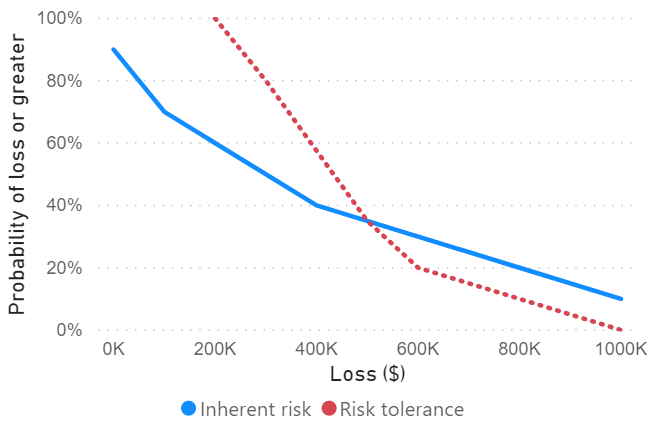
The risk tolerance curve in red shows the maximum level of risk an organisation is willing to tolerate. If the blue line falls below the red, the inherent risk is lower than the tolerated risk. But if the inherent risk is above tolerance, a company may wish to introduce measures to reduce their inherent risk to acceptable levels.
Decision support with our new quantitative method
With the risk matrix, it was very difficult to make budget allocation decisions. We couldn’t really use the matrix to communicate the monetary value of moving a ‘high’ risk to a ‘medium’.
In the graph above, we can see that there is an expected 20% chance of losing more than $800,000 per year due to a data breach. This is beyond the risk appetite of management, so we’d expect that they’d want to invest in a control to reduce the inherent risk. Enforcing two-factor authentication or purchasing data breach insurance may be two possible options. To choose between them, a risk manager would want to know the return on each control. The return is the reduction in expected losses, divided by the cost of implementing the control.
Return on control = (Reduction in Expected Losses/Cost of Control) - 1
To get the values for ‘Reduction in Expected Losses’, we could update our original estimates of probability and impact of a data breach with each of the new controls in place. Implementing two-factor authentication may reduce the likelihood of a costly data breach occuring. Buying insurance could reduce the impact (cost) of a data breach. By running a new set of Monte Carlo simulations, we can see exactly how much the potential losses are reduced with each control in place.
Once the simulations are done, we measure the area under the new loss-exceedance curves and find that the reductions in expected losses are $400,000 and $30,000 for each control.
Implementing two-factor authentication ($150,000 project)
Return on control = ($400,000/$150,000) - 1 = 167% return
Buying data breach insurance ($20,000 per year premium)
Return on control = ($30,000/$20,000) - 1 = 50% return
We can see that the best option above is to implement two-factor authentication. We can even use techniques from finance to estimate the present value of controls that have an ongoing cost (like insurance). Simulating the implementation of two-factor authentication would show that the loss-exceedance curve is below the risk tolerance curve, and is aligned with management’s risk appetite. Decision making for our CEO has been made a lot easier now that they can make direct comparisons between courses of action.
The example above is a simple one. A ‘data breach’ risk would be composed of multiple potential loss scenarios, e.g. employees emailing confidential work home, lost or stolen computers, or hackers gaining access to all customer data. Fortunately our quantitative method allows for risks to be decomposed into individual parts. The parts can even be brought together across a whole portfolio of risks - data breaches, system outages, ransomware attacks. Monte Carlo simulations can combine each risk into a single curve of likelihood and impact.
A new way of thinking about cyber risk - moving past the risk matrix

Quantitative cyber risk modelling unlocks a whole new class of decision making
A common objection to the approach above is that ‘Cybersecurity risk is too complex to model with quantitative methods’. The de facto alternative proposed by critics of the quantitative approach is that cyber security risk can only be modelled in their heads with vague scoring systems. But if the risk is extremely complex, we should absolutely avoid trying to model it in our heads. Simulations for the SpaceX Falcon 9 rockets are complex. But SpaceX engineers aren’t simulating the rocket launches with their ‘expert intuition’. Your pension fund manager will have a wide range of quantitative models to understand the risk exposure of their portfolio. Their portfolios are complex, comprised of stocks and bonds in multiple, often correlated sectors. In order to make sensible decisions about what to be invested in, they absolutely need to quantify their risk exposure in dollar terms.
Cyber security deals with multiple interacting systems, controls and potential loss events. Companies need to roll all of that up into a portfolio to understand their overall risk. It’s not hard to do the mathematics, but it’s really hard to do it in your head. Quantitative measurements of cyber risk are transparent in their assumptions, inputs and outputs. The techniques enable cyber security experts to communicate the risk of cyber loss events in real financial terms.
In the next post, we’ll look at a detailed example and go in-depth on how the numbers above are generated. We’ll look at how to decompose and model risk with a range of loss scenarios, and see how the risk changes with potential mitigation strategies. We’ll also look at running Monte Carlo simulations and generating loss-exceedance curves in Python.