How to load and analyse 48 billion Wikipedia page views with Google BigQuery

This year, the English language Wikipedia has averaged around 8 billion page views per month, making it one of the most visited websites in the world. The first half of 2020 has been incredibly eventful, and I was interested in building a dataset to see exactly which pages Wikipedia users have been most interested in. The Wikimedia foundation publishes archives of hourly page views per article available here. Several sites exist that allow you to compare views between specific pages, but I wanted to see if it was possible to create a full archive for my own usage.

What does the data look like?

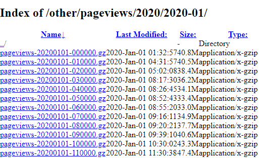
Wikipedia uploads a compressed .gz file for each hour of each day.

The Wikipedia page for Edinburgh had 47 views at 11:00 AM on the 1st of January 2020.

A single file represents one hour of activity on Wikipedia, and contains around 7 million rows and 200 MB of data. Doing some rough calculations, we would need to extract and load 900 GB of data - just for page views in the first half of 2020.

Before we work out how to deal with this large dataset, we need to understand exactly what we’re trying to achieve, and break the problem down.

• We want to download and store all the page views data from the 1st of January 2020 to the 30th June 2020. The hourly page views data is published every few days, so we need to be able to compare what we already have to what is on the Wikimedia page.

• The next step is to combine the page view files into a single source, so we can run queries on the dataset. We will also clean the data at this stage.

• We want to visualise the results of our queries, and present the data in a clear way.

• Finally, every step needs to be automated so the process is repeatable and it’s easy for us to add new data.

Searching through a single uncompressed page views file crashed Notepad++ on my PC. Dealing with ~25 billion rows of data presents an interesting data engineering challenge. The volume of data is too big for my desktop PC to handle, so we’re going to need more computing power.

We only need to move the data once, and run a small number of queries. You wouldn’t go out and buy your own truck just to move house, usually you’d rent one. We’re going to do something similar, by renting the computing power from a cloud provider.

Choosing a cloud provider

The three main players in cloud compute services are AWS, Google and Microsoft Azure. AWS is generally considered to be the most mature with the broadest array of services. Opinions online tend to be mixed as to which provider is ‘best’ for any given use-case. I have some experience with AWS and Azure, and almost none with Google Cloud Platform (GCP). To get a better understanding of Google’s offering, I decided to use GCP for this project. The steps below go how I moved a terabyte of data from Wikimedia to Google Cloud Platform.

Step 0: Create a Google Cloud Project

Before we can access the Google Cloud services, we need to create a project in the Google Cloud console. We set our project name and ID to tc-wiki-2020.

Step 1: Store the data in Google Cloud Storage

Google Cloud Storage is an Infrastructure as a Service (IaaS) platform for storing files on Google Cloud Platform. It works in a similar way to Amazon S3 storage, where users can store objects in buckets. Each bucket has a unique, user-assigned key. Buckets and objects can be addressed using HTTP URLs. For example, the bucket tc-wiki-2020-bucket and object pageviews-20200101-000000.gz would be accessible through:

https://storage.googleapis.com/tc-wiki-2020-bucket/pageviews-20200101-000000.gz

We created the bucket in the Google Cloud Console.

The Python script below automates the transfer of page view records to Google Cloud Storage. The script does the following:

1. Read the page view URLs on Wikimedia and compare to what has already been uploaded to the Google storage bucket.

2. For files that haven't been uploaded yet, add the names of the files to a list.

3. Loop through the list, and download each file one at a time.

4. Add the downloaded file to our Google storage bucket, and delete the local copy.

The first input ‘creds.json’ for the functions above is a credentials file, which can be generated by following the instructions on how to authenticate with a Google Cloud API. If you’re following these steps yourself, keep the file somewhere safe as it provides access to your Google Cloud account.

The ‘months_urls’ is a list of the root URLs for each month of interest. Once we have the inputs, we can run our functions to upload the page view files.

Step 2: Load the data into Google BigQuery

Now that we have all the compressed page view files in Google Cloud Storage, we need a way to combine them all together and run queries. BigQuery is Google’s serverless data warehouse product. ‘Serverless’ in this case means that we don’t need to deploy any computing resources ourselves, like virtual machines. We simply tell BigQuery where our data is stored and query the data with SQL. Instead of paying for all the expensive database hardware and infrastructure upfront, we just pay for storage and per query (more on this later).

Before we create a table, we need to create a dataset within BigQuery. The dataset must have the same geographic location as our source data europe-west2 (London) in our case. The dataset was created using the Cloud Console and was named views.

Now we can create a table with Python, using the BigQuery API.

The Python code and SQL code below was adapted from Felipe Hoffa’s blog post outlining a clever way to load the data into BigQuery. The data gets parsed line by line, and is not split into columns at this stage. Because the configuration requires a delimiter, the delimiter u’\u00ff’ was chosen to be as obscure as possible to avoid any data loading issues. BigQuery natively supports .gz files, so we don’t need to decompress the source page views files before loading.

Lets see what the data looks like:

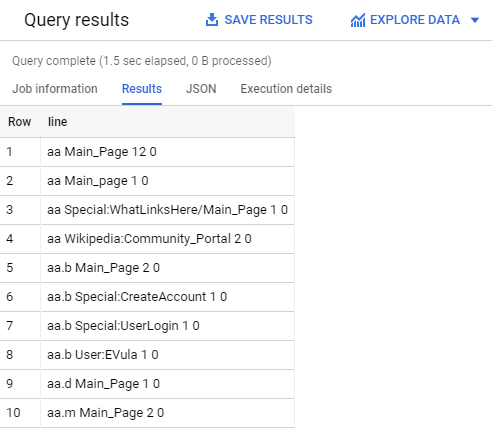
Google allows us to create the table as a federated table - one that can be directly queried even if the data isn’t stored in BigQuery. Once we have the view of the raw data defined, we can create another view that uses regex to extract the columns of interest from each line:

What does the new view look like?

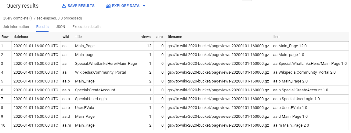
The table above looks like something we can work with. At the moment, the data is being directly loaded from the .gz files in Google Cloud Storage. This approach saves us money, as BigQuery charges around £5 per TB of data queried. But if we import the data into BigQuery, it gets converted into a much more efficient internal representation. You can read more about Capacitor, BigQuery’s columnar storage here.

Step 3: Create tables with the data

Now we create a new dataset in our project called ‘wikipedia’ to keep the tables separate from the views. Next, we run the query below to build the page views table. Partitioning the table by date divides the very large page views table into smaller more manageable chunks. Adding the ‘require-partition-filter’ argument forces us to specify a date range when querying the table. Filtering saves money when writing queries, as the more data we query, the more the query costs.

Finally, we load the data from the view into our new table:

The WHERE clause specifying dates from 2001 onwards was necessary as our table forces date filters for any query run.

The WHERE NOT EXISTS clause ensures that the we only add new files into the table, so we can re-run it if we have new data.

Step 4: Filter the data we don’t need

The next step is to filter out the pages and data not relevant to our analysis. We’re focusing page views for the English Wikipedia pages. The English language pages visited from a desktop computer are flagged as en in the wiki column and en.m for pages visited on a mobile device.

We’re only interested in daily views, so we will group the hourly views by day at this step. We’re excluding some of the default and error pages that tend to have high view counts, but aren’t useful for our analysis.

This ends up being one of the more expensive queries, as it needs to run over the entire pageviews_2020 table in order to filter by English pages only. Once we have the smaller table, our subsequent queries are over a smaller dataset and are comparatively less expensive.

In Wikimedia’s article on the top 10 pages of 2019, they said that ‘any article with less than 10% or more than 90% mobile views was removed, as it is a strong indicator that a significant amount of the page views stemmed from spam, botnets, or other errors.’ When looking at the the data on a day by day basis, the top ranked pages usually tend to have as many, if not more mobile views than desktop views. We can see below that the page for ‘Media’ has a huge spike in mostly desktop views on the 4th and 5th of January:

Step 5: Rank the pages by daily view count

The final step is to add a ranking for each page on each day. The ranking will give a consistent way to filter for the ‘top n’ pages viewed for a given date. For our daily ranking, we’ll exclude pages that look like they had their page views boosted by bots. We’ll do some data cleaning of the NULL values at this stage, and add a column for the ratio of mobile views to desktop views:

Conclusion

Now we have a data pipeline to load new page views files, clean the data and rank the popularity of the pages each day. Google Cloud Storage and BigQuery have worked well, and we’ve managed to load and process all of the 2020 page views data with a total bill of around £7. Considering that Wikipedia is one of the most visited websites in the world, it’s pretty amazing that we can build these kind of data analysis pipelines so cheaply and easily using cloud compute resources. These days, individuals and businesses have a huge amount of computing power at their disposal with cloud computing.

In the next post, we’ll be looking at extracting the most viewed pages of people in 2020 and building a data visualisation.